
DonVK’s second article deals with the verification of the DrBA spherical wave horn calculator and BEM simulation model construction. Only the round mouth spherical wave horn was initially used for comparison to published works. Additionally, the effect of adding a roll-back section or even more a merge of the roll-back section with the inner horn wall will be discussed. As already mentioned in the original patents, the continuation of the horn profile beyond the mouth plane has positive effects and leads to more even results.
Baseline Verification
DrBA Calculator and BEM Simulation
by DonVK
1.0 Introduction
This document describes the initial checks that were performed to verify a baseline for horns generate using the DrBA SWH calculator [1] with BEM simulation models in 4Pi space using ABEC [3].
2.0 Spherical Horn Contour Baseline
The round spherical horn (aka the Klugelwellen by Klangfilm) is a well established horn contour that will be used for the baseline test case. There are published examples [4,5] of how this basic horn should perform. Our results are compared to published results to verify that the new DrBA calculator [1] and new BEM simulation models are functioning properly. Figure F.1 shows our test case horn.
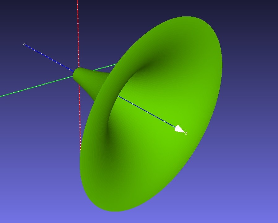
Figure F.1 Spherical Wave Horn (SWH), Fc=400Hz, 35mm Throat
2.1 Horn Profile Comparison
Horn Response [2] is an established calculator that can provide an independent contour of a round spherical horn and we can export the profile coordinates to a CSV file for comparison. The CSV file can also be used to generate a contour in FreeCad [6] so that it can be simulated as well.
The DrBA horn profile and HornResp profile are virtually identical as seen in Figure F.2 so we can say it’s a spherical horn. HornResp’s simulation outputs are based on a simplified model so it will be “close” but not exactly the same as the BEM simulation.
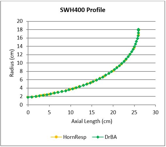
Figure F.2 Profile Comparison, Fc=400Hz, 35mm Throat
3.0 BEM Simulation Model
3.1 Model Symmetry
The horn can be simulated in ABEC as a full model (no symmetry) but the model will be large (#elements) and the simulation time can be long. So the basic horn was simulated with no symmetry and ¼ symmetry, to check if there was any reduction in the results quality. It turns out that cutting the mesh actually increases the mesh resolution along the cut edge because the cut mesh elements (facets) are now smaller. The ¼ symmetry model (Figure F.3) solution did not affect the quality of the results.
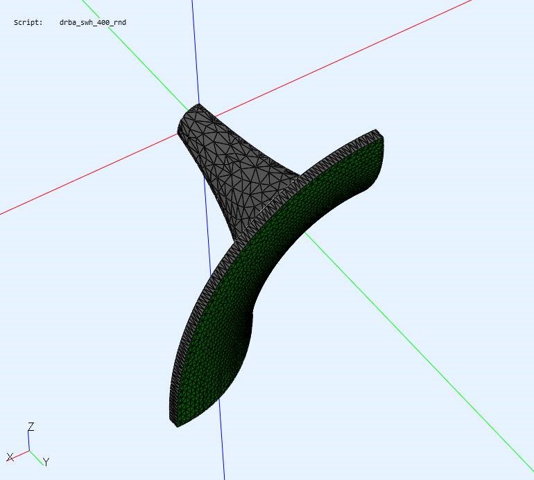
Figure F.3 Spherical Wave Horn (SWH), ¼ Symmetry Mesh, Fc=400Hz, 35mm Throat
3.2 Mouth Interface, Subdomain Boundary
The ABEC [2] BEM simulation model (Figure F.4) is divided into an internal horn space (domain, green) and the external 4Pi space (grey). The domain boundary is user defined by a mesh surface (purple). The boundary should be near the horn mouth but the proper shape and exact location have to be determined. Several shapes (planar, rectangular box, cylinder, mouth perimeter concave, mouth perimeter convex) were tried at or around the mouth to check the output result’s sensitivity to both boundary shape and location. The boundary choice effects the simulation output results.
The subdomain boundary (purple) needed to be at the mouth apex to provide a simulation result that matches the published results [4,5]. This is also intuitive because the physical boundary of the horn (mouth apex) should be consistent with the subdomain boundary.
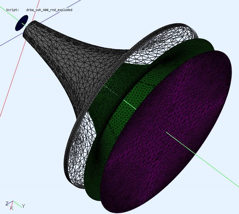
Figure F.4 SWH Model, Exploded Model Component View, Fc=400Hz, 35mm Throat
3.3 Driver Membrane
Some original simulations were done with the ABEC built in diaphragm generator (flat membrane). During initial testing, some artifacts in the results were noticed as the simulated frequency increased. In a round horn there should also be symmetry between the horizontal and vertical polars. The built in diaphragm generator cannot align perfectly to the throat mesh (edge, vertices) and this is a problem at higher frequencies. A new flat disc driver membrane was created in FreeCad [6] that exactly matched the throat mesh. The driver membrane was later mesh constrained with a small edge length that improved the simulation polar symmetry and high freq. performance. Figure F.5 shows the membrane (blue) mesh edge and vertices aligned to the throat even when the interior mesh resolutions are different.
The idealized membrane can be driven in ABEC using a simple constant velocity or constant acceleration sources. Both drive types are modeling simplifications to study the horn characteristics without having to provide a full LEM compression driver model. The drive source choice does not affect the radiation impedance calculation or any normalized plot results that we have provided. We have used constant velocity for consistency with other published results and it seemed reasonable as it’s used for impedance calculations (ie. pressure/velocity).
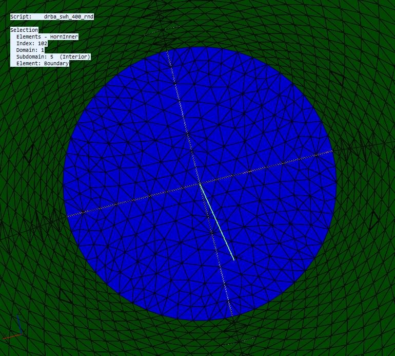
Figure F.5 SWH Model, Driver Membrane (Blue), Fc=400Hz, 35mm Throat
3.4 Mesh Size and Quality
The mesh fields are generated by tools [7,8] that are constraint driven but you cannot predict the exact mesh pattern apriori. You can determine if you have a sufficient quality mesh when there are no troublesome artifacts in the mesh surface or the BEM output results. The minimum initial requirement is to set the mesh edge length or mesh frequency based on the max simulation frequency. It is an important factor as the mesh determines the model size (#elements), simulation time, results quality and max usable simulation frequency. The different mesh resolutions can be seen in Figure F.4, and it was meshed using Driver=5mm, Inner Horn=10mm, Mouth Interface=10mm, Outer Horn = 20mm.
4.0 SWH Round, Simulation Results
The SWH horn seen in Figure F.6 was simulated using ABEC [3]. You can see the ¼ symmetry cut line even though the image is shown in full symmetry. The simulation results match published results [4,5].
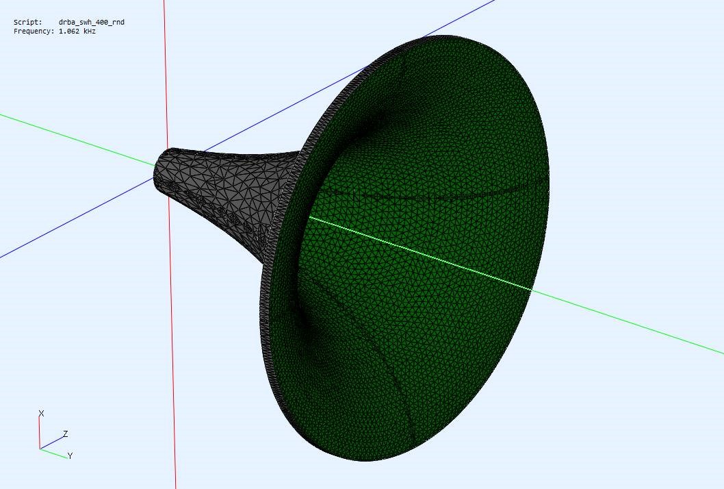
Figure F.6 Spherical Wave Horn (SWH) Round, 1/4Symmetry, Fc=400Hz, 35mm Throat
Figure F.7 show the near field SPL fields [400Hz, 1Khz, 2.6Khz, 5.2Khz, 9.1Khz, 16Khz] and you can see well behaved wavefronts and the expected polar narrowing at higher freq. There is very little radiation around the horn mouth side walls and there is some diffraction from the sharp mouth edges.
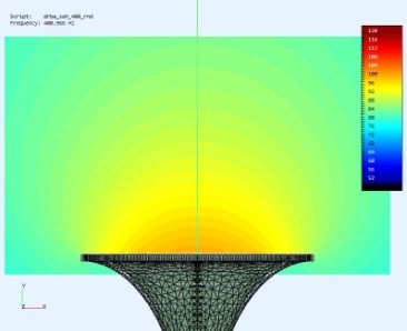
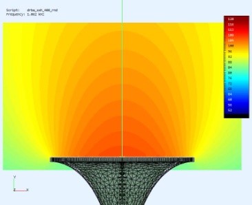

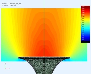
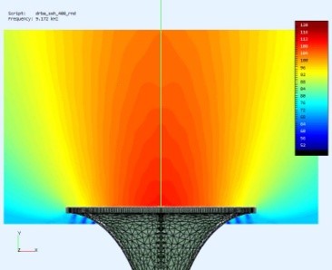
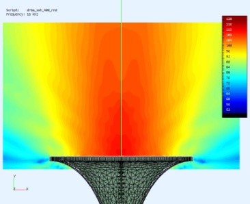
Figure F.7a – F.7f SWH Round, Near Field SPL Field Diagrams, f=[0.4K, 1K, 2.6K, 5.2K, 9.1K, 16Khz]
Figure F.8 shows the radiation impedance ripples for this type of horn and it also matches the published results. We can also see there is an impedance ripple from mouth reflections and diffraction. We can also see the characteristic round SWH SPL polar dip at 1.5Khz and a bump at 2.5Khz for this Fc=400Hz. A more detailed ½ polar contour view is provided in Figure F.9.
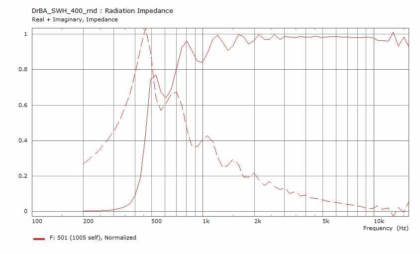
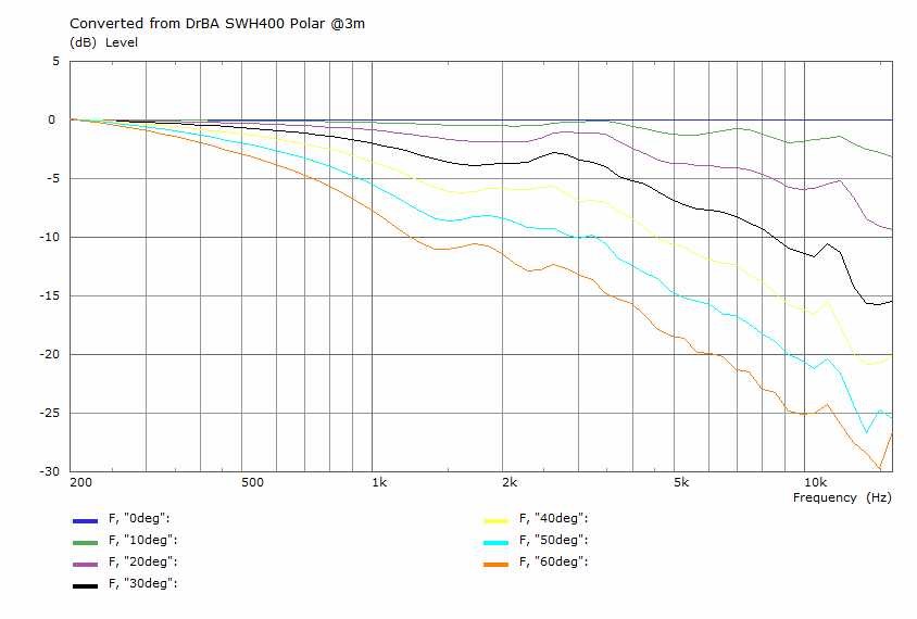 Figure F.8a-F.8b SWH Round, Radiation Impedance, and Polar Curve Plots @3m, f=200Hz-16Khz

 Figure F.9a-F.9b SWH Round, Full Polar Plot and Magnified 1/2 Polar Plot
5.0 SWH Round + RollBack Simulation Results
The mouth reflections and diffraction can be reduced by sufficient rollback as shown in Figure F.10 and F.11. The horn wall is continuous but the BEM model has the mouth interface declared at the horn apex which is also where the horn interior (green) rolls over and becomes the horn exterior (grey).
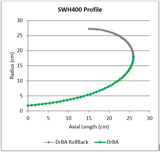
Figure F.10 SWH Round + Rollback, Profile Comparison, Fc=400Hz, 35mm Throat
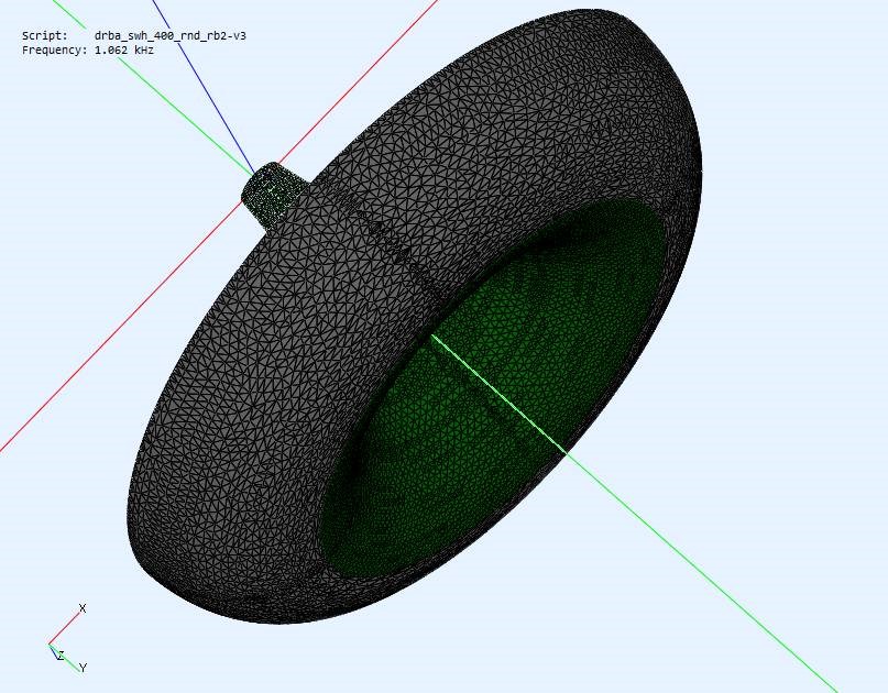
Figure F.11 SWH Round + Rollback, Fc=400Hz, 35mm Throat
Figure F.12 shows the rollback improvements in the quality of the SPL field at higher frequencies as there is a better impedance match from less reflection. The diffraction at the edges has also been reduced. The rollback does not affect the basic polar pattern of a round spherical horn. Figure F.13 shows the improvements in the impedance match as the ripples are mostly gone and we have a smooth impedance curve. Figure F.14 shows the polar contours which have smoothed considerably.
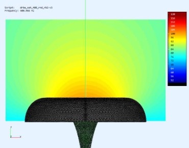

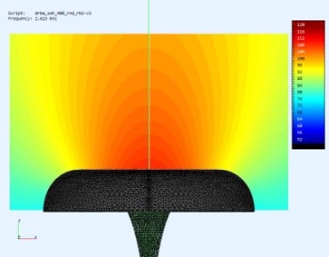
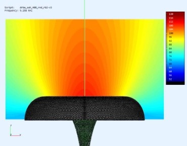
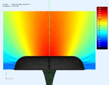
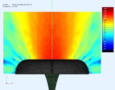
Figure F.12a-F.12f SWH Near Field SPL SWH Round + Rollback, f=[0.4K, 1K, 2.6K, 5.2K, 9.1K, 16Khz]
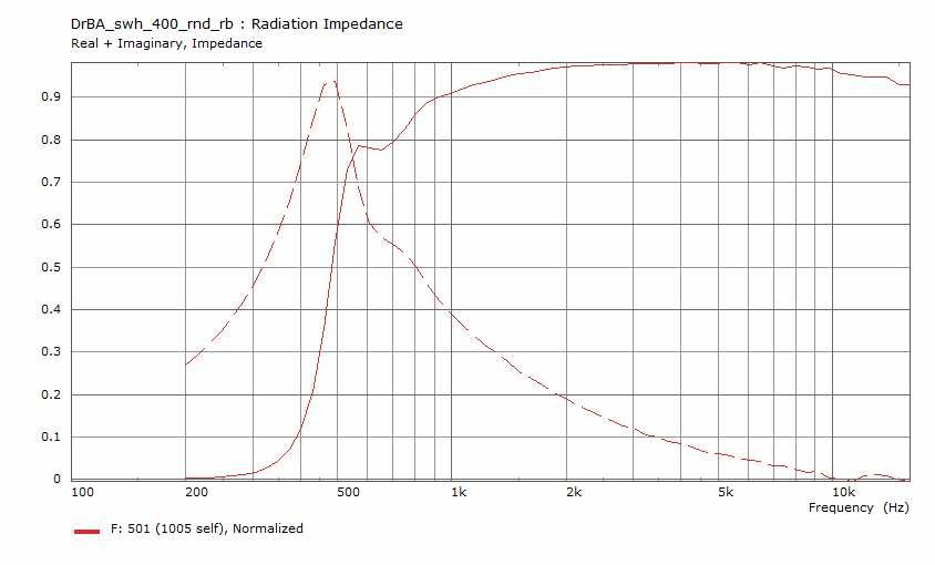
 Figure F.13a-F.13b SWH Radiation Impedance, Polar Curve Plots @3m, f=200Hz-16Khz

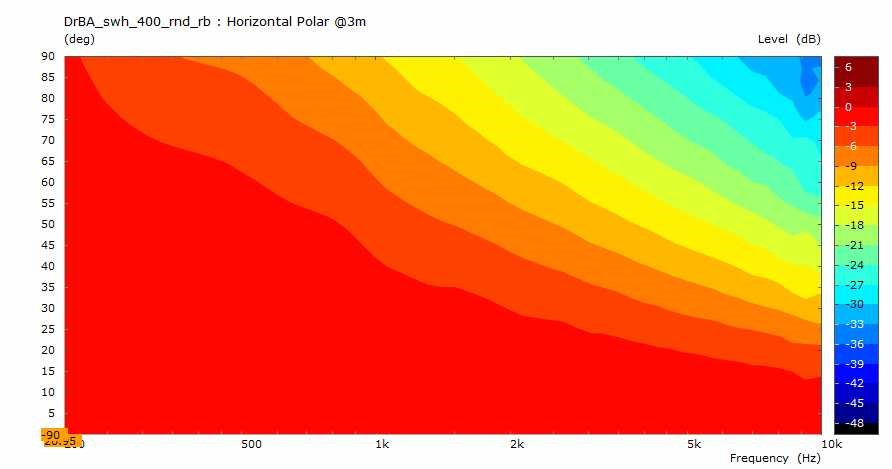 Figure F.14a-F.14b SWH Round+Rollback, Full Polar Plot and Magnified 1/2 Polar Plot
6.0 SWH Round + RollBack + Merge Simulation Results
Here the rollback is further modified to merge back towards the inner horn and throat. The merge further extends the outer horn surface and makes the horn more slightly more compact while further smoothing the output. The basic polar contour is similar to the previous round horns and is again further refined in smoothness.
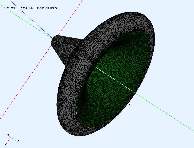
Figure F.15 SWH + Rollback + Merge, Fc=400Hz, 35mm Throat

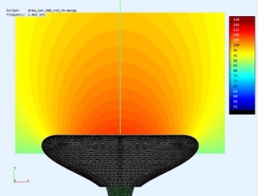
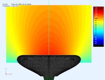
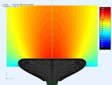

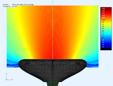
Figure F.16a-F.16f SWH Near Field SPL SWH Round+Rollback+Merge, f=[0.4K, 1K, 2.6K, 5.2K, 9.1K, 16Khz]
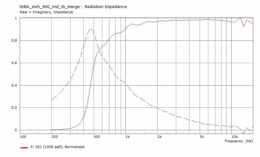
 Figure F.17a-F.17b SWH Round+Rollback+Merge, Radiation Impedance, Polar Curve Plots @3m, f=200Hz-16Khz
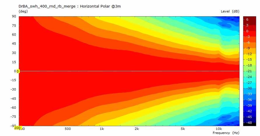
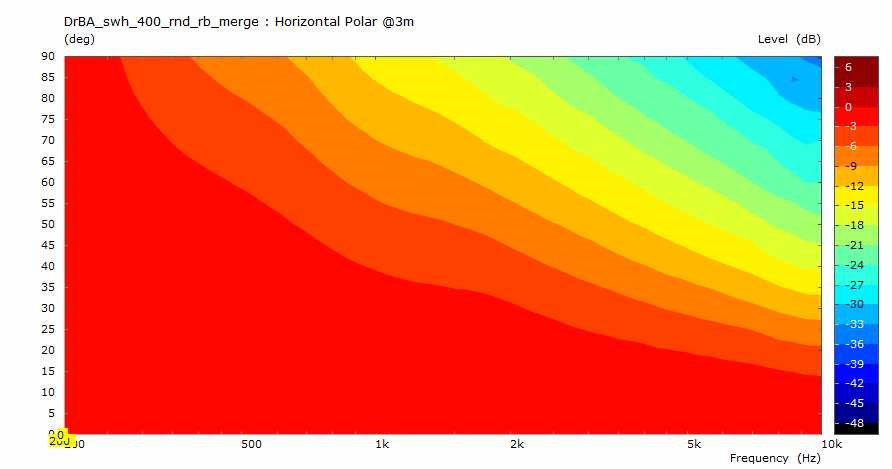 Figure F.18a-F.18b SWH Round+Rollback+Merge, Full Polar Plot and Magnified 1/2 Polar Plot
References
[1] Software, DrBA Calculator, https://sphericalhorns.net/
[2] Software, Horn Response, David McBean, http://www.hornresp.net/
[3] Software, ABEC3, RandD Team, http://www.randteam.de/ABEC3/Index.html
[4] SWH published results, http://kolbrek.hornspeakersystems.info/index.php/horns/bem, plots #101,#102
[5] SWH published results, Horndesign und Hornoptimierung mittels BEM, Michael Makarski, Institut fur Technische Akustik, RWTH Aachen, ref Figure 7.6
[6] Software, Freecad, https://www.freecadweb.org/
[7] Software, Gmsh, http://gmsh.info/
[8] Software, Meshlab, http://www.meshlab.net/