
In this article I will present a step-by-step guide transforming the point cloud exported from my spread sheet calculator into a 3D triangular mesh. Although my first implementation of a simple 3D visualization was done within Excel, I started looking for a tool that can convert point clouds into 3D printable files. After a first euphoria, however, I quickly realized that an existing and properly looking stl- or ply-file does not necessarily mean that you can print it that way directly. But that’s another story.
If you search the web for point clouds, you will inevitably come across a freely available software called MeshlabTM (http://www.meshlab.net). After some initial tests this software worked very well for my purpose, so I have adapted my spread sheet calculator that the exported point clouds can directly be imported without any change by MeshlabTM. I will now describe the whole workflow by meshing the point cloud of a spherical wave horn with 400Hz cut-off, a stretch factor of 1.5 and 1.4″ throat radius. The header line of the calculator shows the corresponding input parameters:

There are several parameters but most of them do not need to be changed and it may look more complicated than it actually is. I refer to the README tab of the spread sheet for a more detailed parameter description. Just point your attention to the green input fields. The projection factor of 3 disables stereographic projection in this case as it is larger than 2. It is also obvious that a slight super ellipse transformation is applied with a Lamé exponent of 2.333. The stretch option 5 was already described in a previous post. The f(x) arc length steps is an important parameter to influence the number of vertices created during meshing. A larger value means a finer mesh. But larger is not always better. Values between 30 and 60 are reasonable and beyond 60 may give a finer mesh but could also produce problems during the meshing. If the resulting mesh is still showing artifacts then it might be a workaround to change the step size and simply generate a different point cloud. The calculator can either be started by clicking on the diagram on Sheet1 or over the Developer Options. Before the point cloud calculation section is started two property windows appear which inform about the horn and stereographic projection properties:
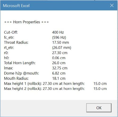
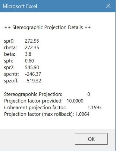
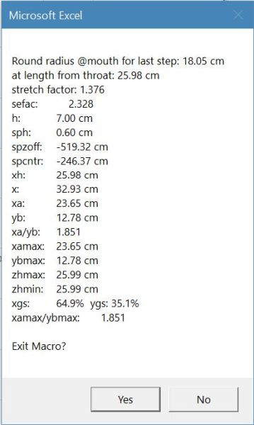
Just click OK in both windows to continue. Now, the calculation is initiated and the horn profile gets printed into the diagram. Once the mouth region is reached, another window with several run parameter values appears asking if the calculation should be terminated at this point. If No is selected the calculation continues into the roll-back region. But in this case Yes is the choice and the calculation is stopped at the mouth of the horn.
The last window is important and needs to be answered with Yes if the export of a point cloud is desired which is our intention:
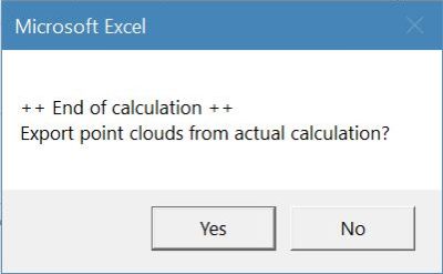
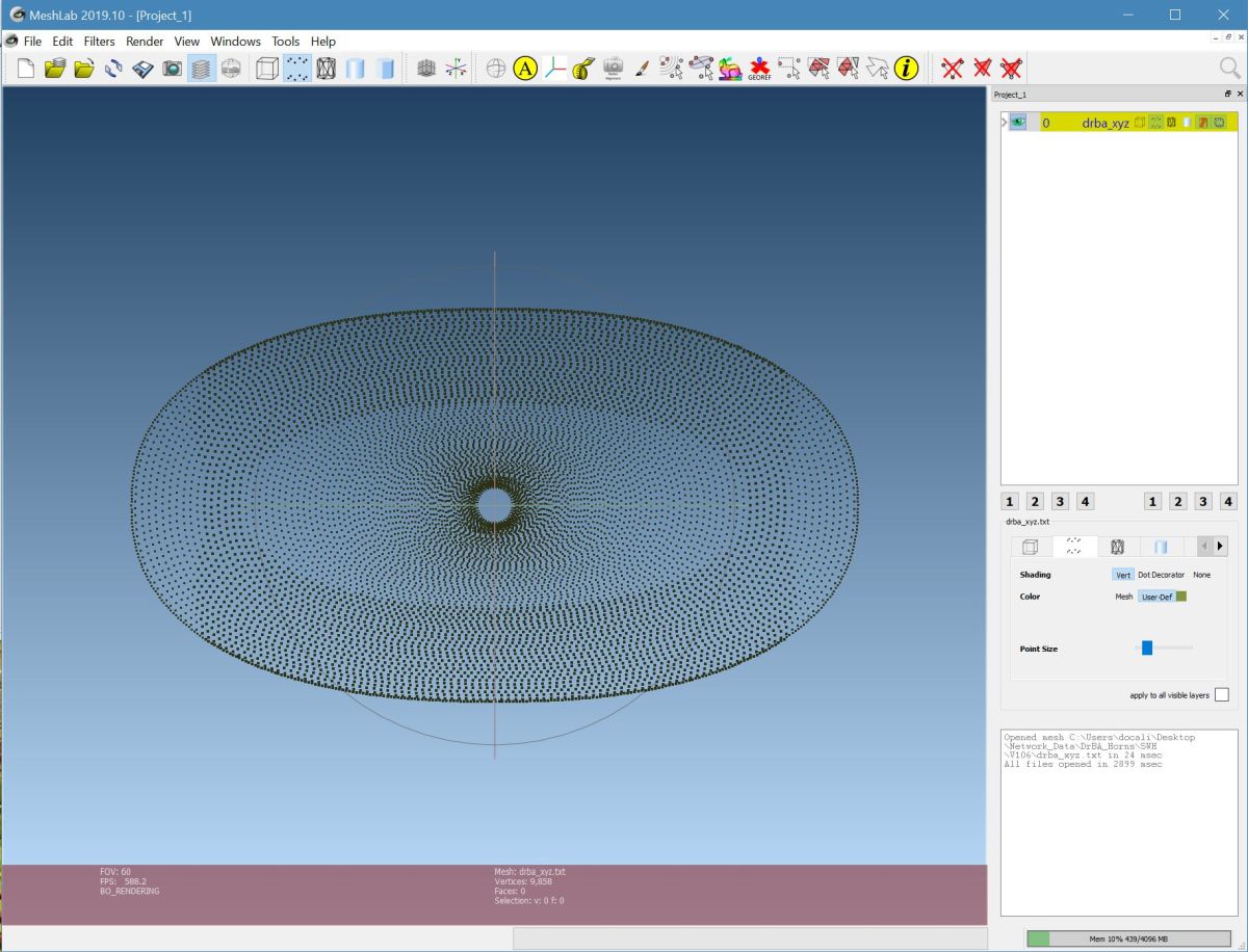
The result will be stored in the local working directory as plain text file drba_xyz.txt. Now, it’s time to open MeshlabTM and import the point cloud file:
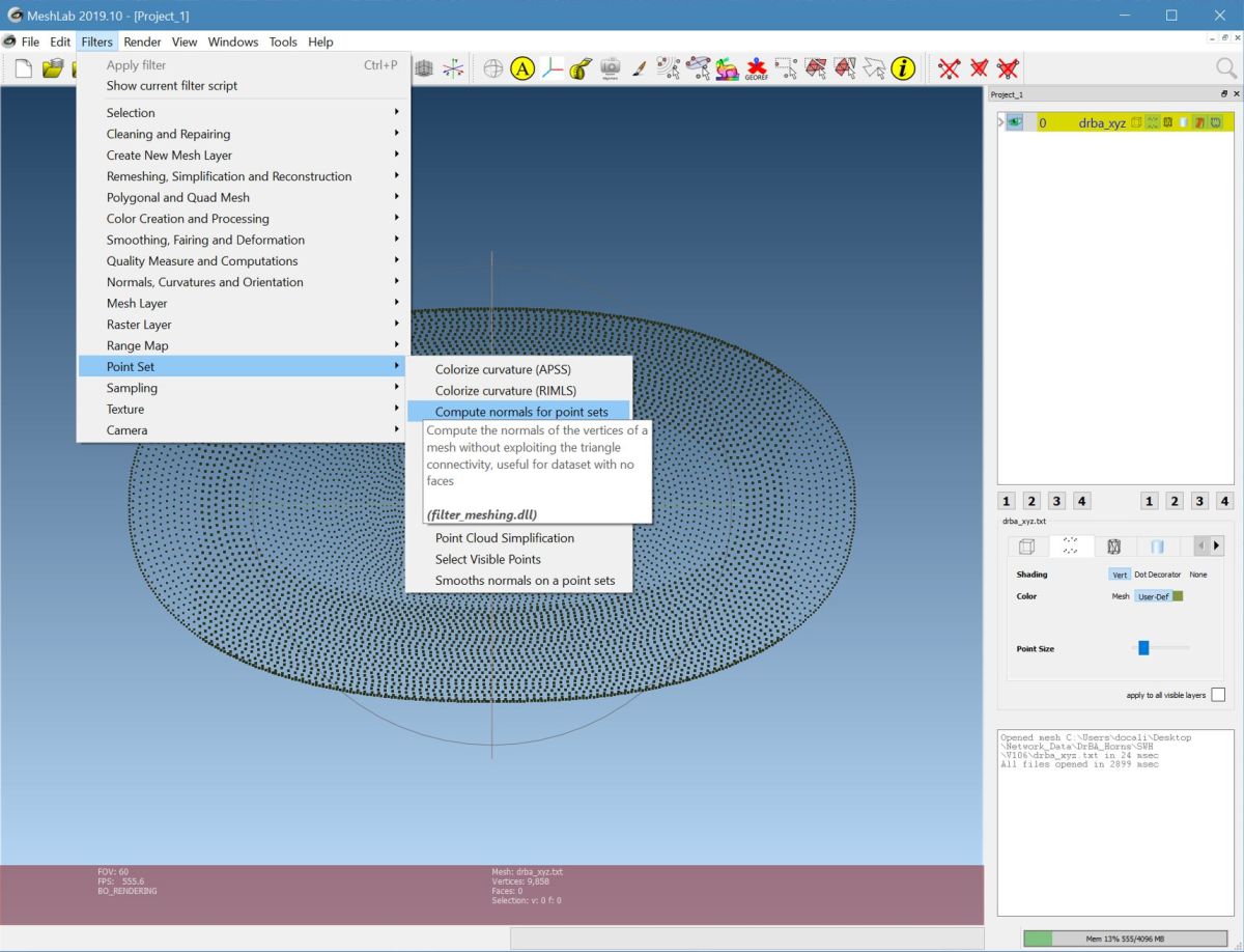
The next step is to compute the normals for the point sets:
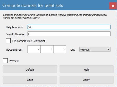
I prefer to choose a slightly higher value 30 for the neighbors than the standard value of 10. Simply click apply and close the window:
After this step the points get marked in a different color:

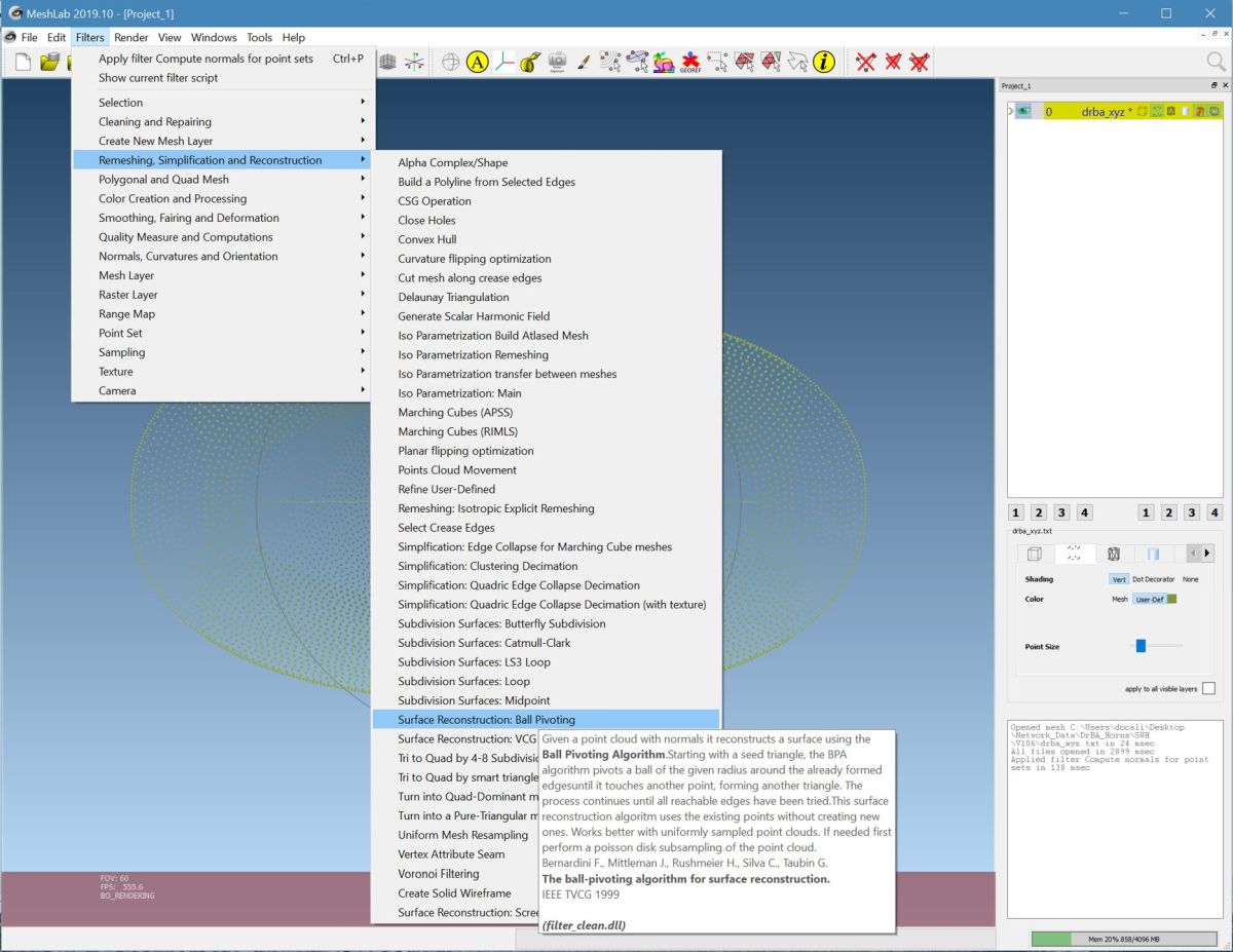
This was already everything needed to start the surface reconstruction. The most reliable algorithm for this purpose has been found to be the Ball Pivoting algorithm:
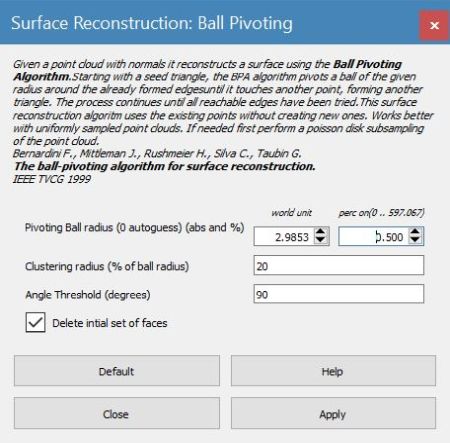
If the ball radius is set to zero the program is doing an autoguess of the ball radius. This already works very good in many cases. If still holes remain in the surface the “Delete initial set of faces” option can be marked and the ball radius can be set to 0.5 and stepped as long as the surface get’s closed.
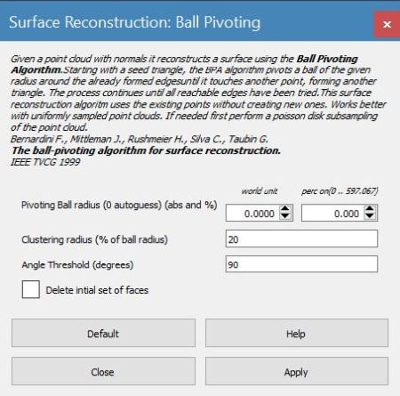
Changing the clustering radius or the angle threshold may help for some special cases. The progress and results of the current action can be seen in the info window right down:

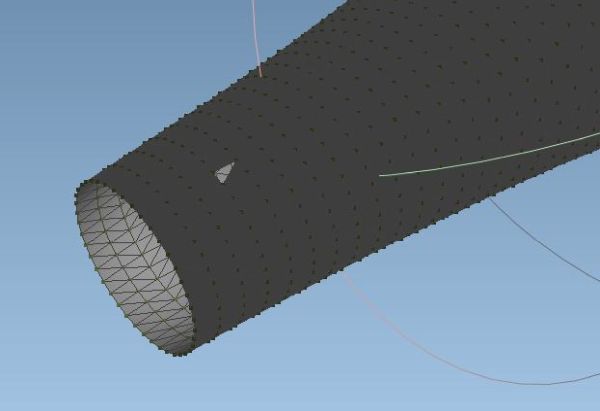
Here is an example for the autoguess which has still a hole in the throat region:
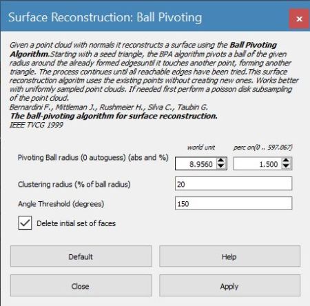
Setting the ball radius to 1.5 was a better option here and produced a fully closed surface without any holes:
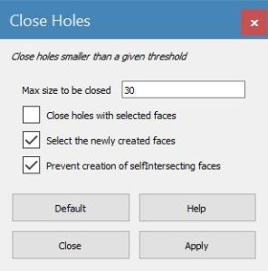
Another way to close holes is to use a special dedicated option for such a task. But do not choose the max size too large as this could accidentally close the throat. As MeshlabTM does not have a meaningful roll-back mechanism up to now this could mean that you have start from scratch and re-import the point cloud.
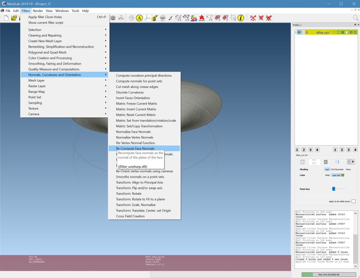
The last step before exporting the result is to re-compute the face normals:
Now, we are ready and are able to export the 3D file for which I usually prefer the ply-file format. Leave all settings as shown here:

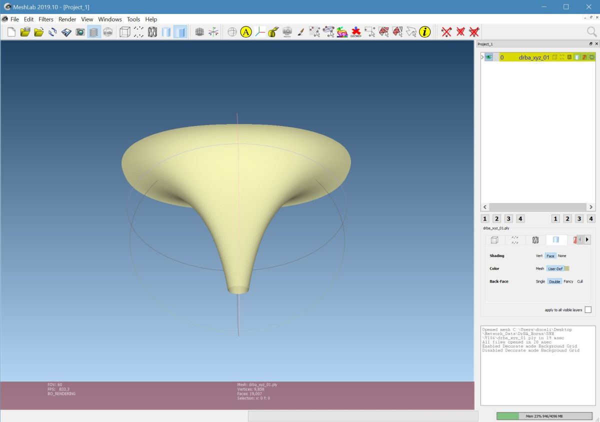
If the ply-file is imported again the final shape of the horn becomes more obvious. Be aware of the settings in the right control window:
That’s it!