In the previous article I already presented some basic information about the semi cubic parabola (Neile parabola) and why I got interested in this mathematical function (Link1). The initial intention was indeed to calculate curved fins with equal path lengths (arc length). But first, a verification of this mathematical function for it’s use as a horn profile should show acceptable results because the two outer Neile parabolas define the outer horn contour. Within most of my previous horn calculators two different functions in two orthogonal planes were sufficient to generate a point cloud by blending the two functions together to form an ellipse at each iteration step along the horn axis. But I decided against this procedure because in the meantime I could make some experiences how to generate a point cloud for radial like horns which can quite easily be made out of wood with a CNC milling machine. The reader should be familiar with the basic blueprint of a radial horn. For the use of the Neile parabola to this type of horns some things are a little bit different as we have no exact radial expansion from a pre-defined point of origin of the profile. In this article I will describe the basic steps how to create a William Neile horn and show some initial BEM simulations as proof of concept for this type of horns.

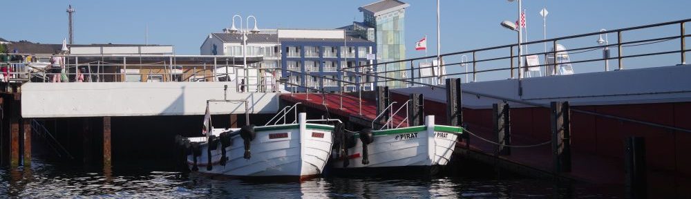
As already described the use of several equally distributed Neile parabolas at throat and each with the same arc lengths build a construction wave front in the horizontal plane which is at the same time the boundary of the horn at each iteration in this plane. So far as I know horns which have equal path lengths assumed to the boundaries in the expansion direction are called isophase horns. Let us call the Neile horn quasi isophase as it is unknown if the real expansion in each direction will occur as assumed.

Construction Wave Fronts at equal path lengths

What can see from the picture is that the construction wave front is nearly flat at throat and bends because of the same arc length constraint. For me this looks quite similar as a real wave front would behave if we assume the same velocity of sound in every direction. In order to make this 2D shape a 3D shape we need a height at each iteration which could either be another native Neile parabola or the height is calculated to follow a certain expansion formula of the bended 2D mouth construction wave front.

What has always bothered me are the sharp edges of most radial horns and this should be avoided. But any approach to accomplish this should be kept as simple as possible. I ended up with this algorithm:

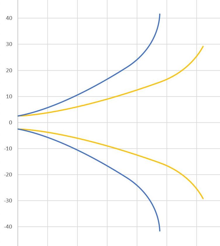
William Neil Horn hrz and vrt Profile Expansion

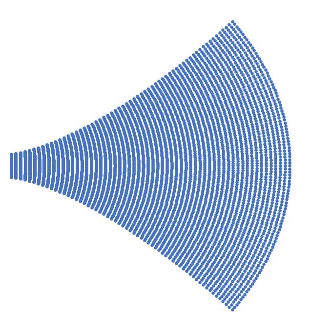
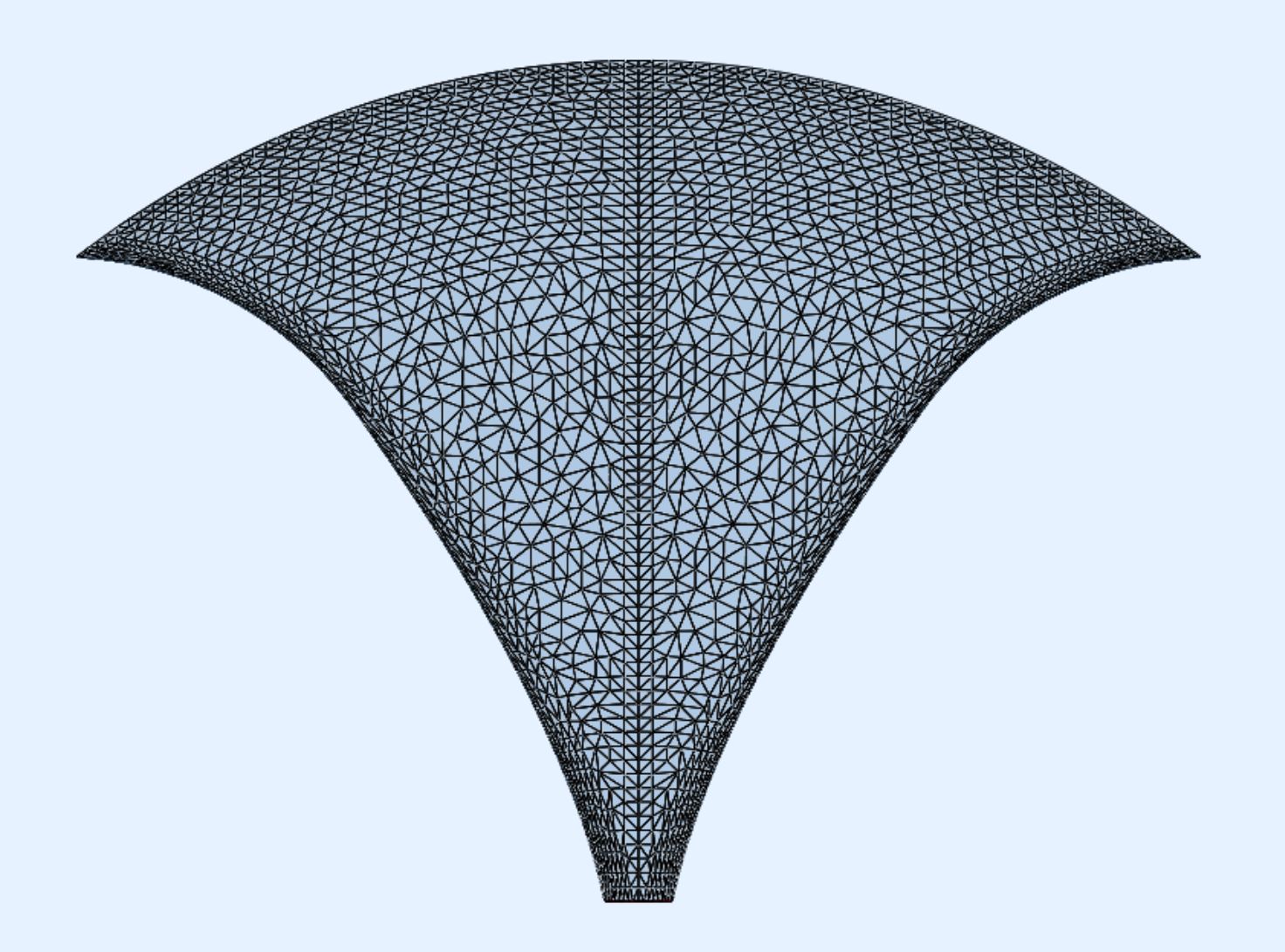
The initial round throat surface is kept throughout the horn from throat to mouth by dividing it into 4 equal pieces and by adding the corresponding horizontal and vertical rectangular surface elements. As the horizontal shape is curved the real challenge was to rotate the circular sections from a local to the global coordinate system to have them properly aligned. Coordinate transformation is no big thing but to get this numerically smooth was tricky. Generally speaking, the throat divided into four pieces become to rounded edges of the horn along the horn axis:

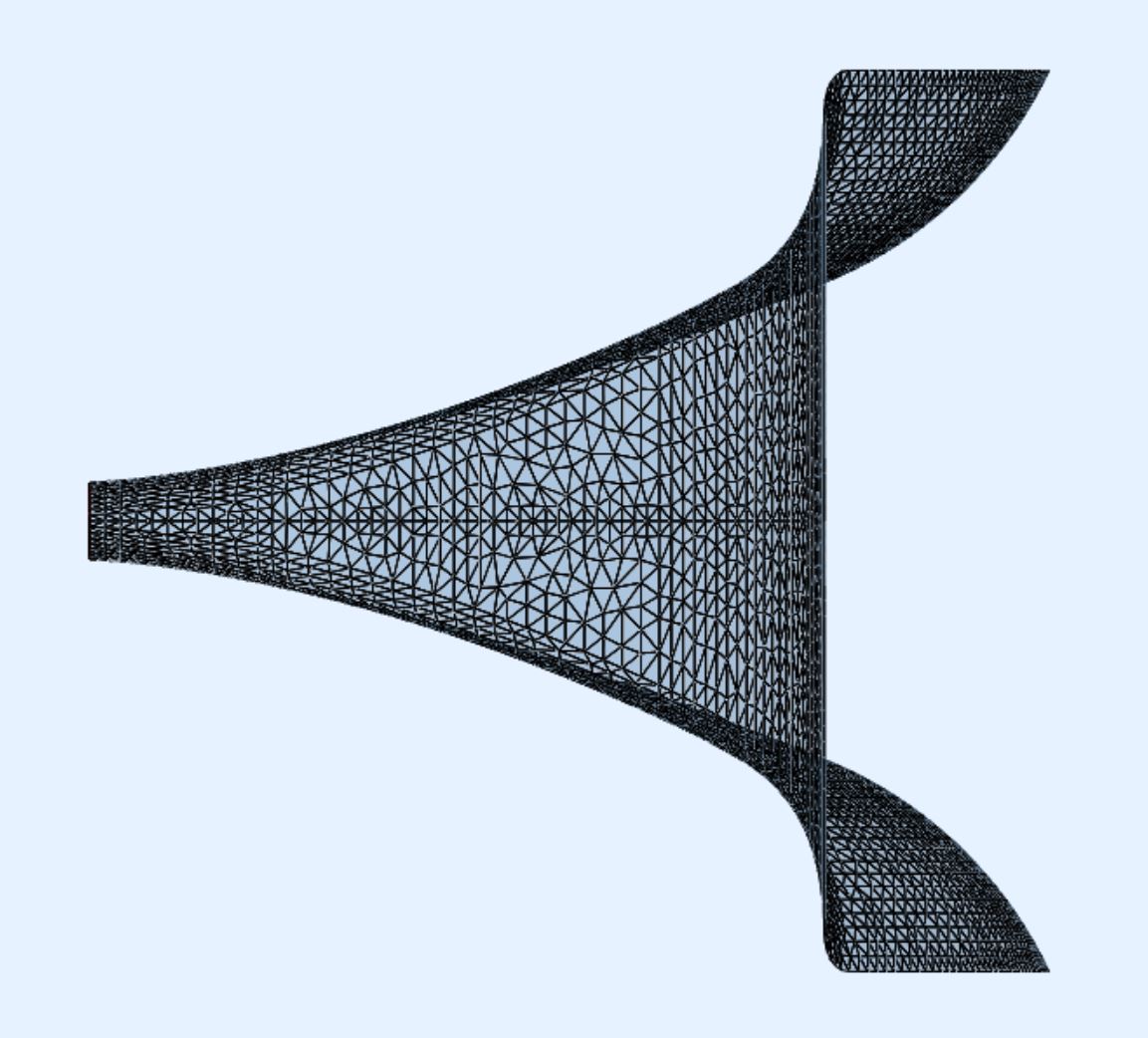
This mesh for demonstration is taken from the BEM model. Only 1/4th of the mesh is needed for the calculation because of symmetry reasons. The model investigated uses two different Neile parabolas for the vertical and horizontal expansion without respecting any construction wave front expansion.

Therefore it is not expected to get exponential horn loading figures. As can be seen from the profile overview the Neile parabolas are terminated each with a different radial end flare to avoid midrange narrow. It is known since a long time that such a termination is beneficial to the overall horn performance. This waveguide was designed having the Celestion Axi2050 in mind which should be an adequate mate for such a large waveguide. The throat diameter is therefore 2″ and the length about 62cm. Really large!

Some words about the BEM simulations for which AKABAK was used and the “constant something” drive used. A good post about constant velocity or constant acceleration can be found here: Link_to_diyaudio. As for all previous BEM simulations shown on my page constant velocity drive was applied. Anyway, if the polar contour results are normalized they should be independent of the drive type. However the actual SPL level prediction requires an appropriate driver model.

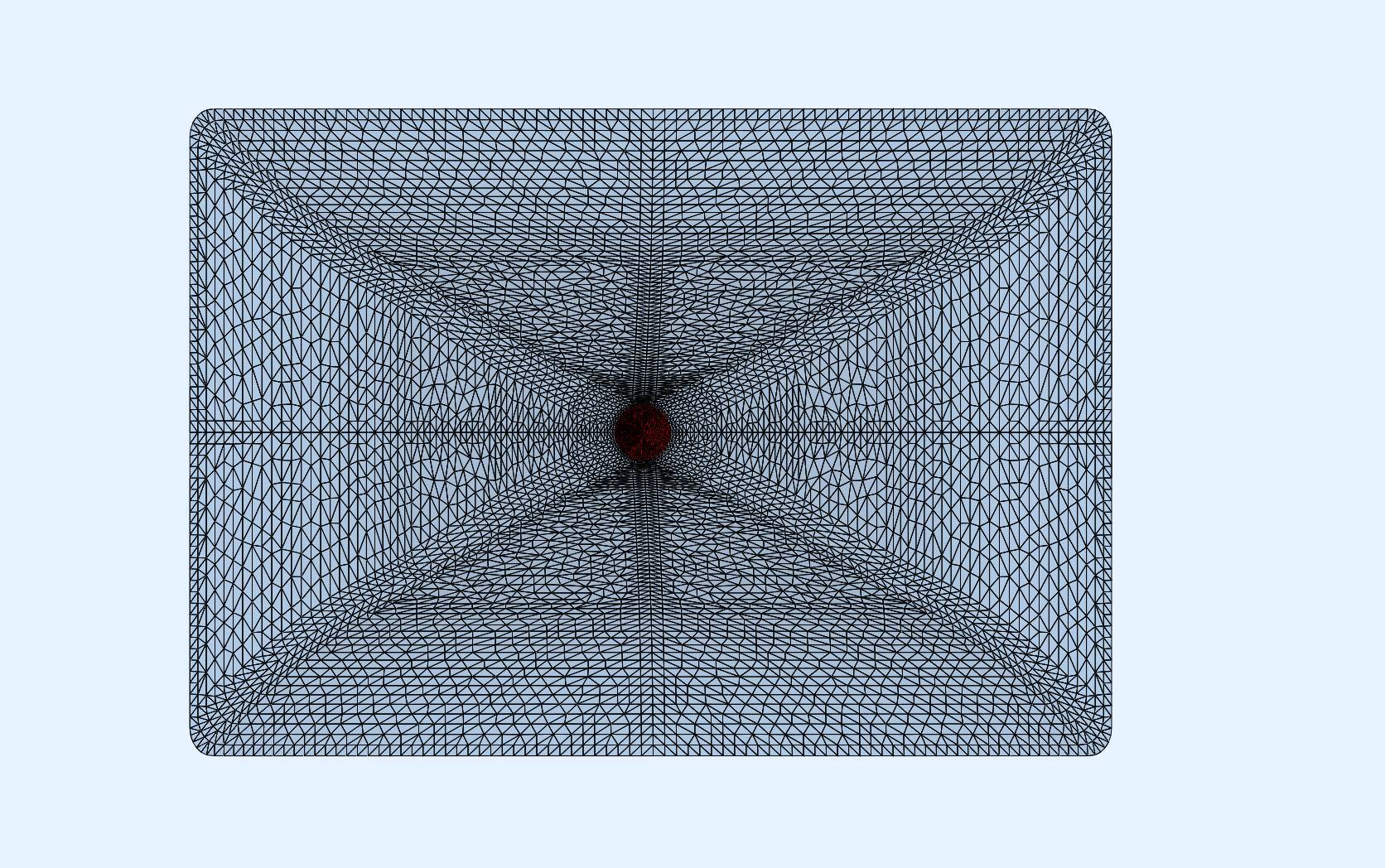
The simulation was done as free-standing waveguide showing the shifted elements for demonstration in the next picture. There are two subdomains, “inner horn” and “free space” and the interface  which connects both subdomains at the mouth plane. The resolution of the outer horn surface can considerably be reduced to save computation time:

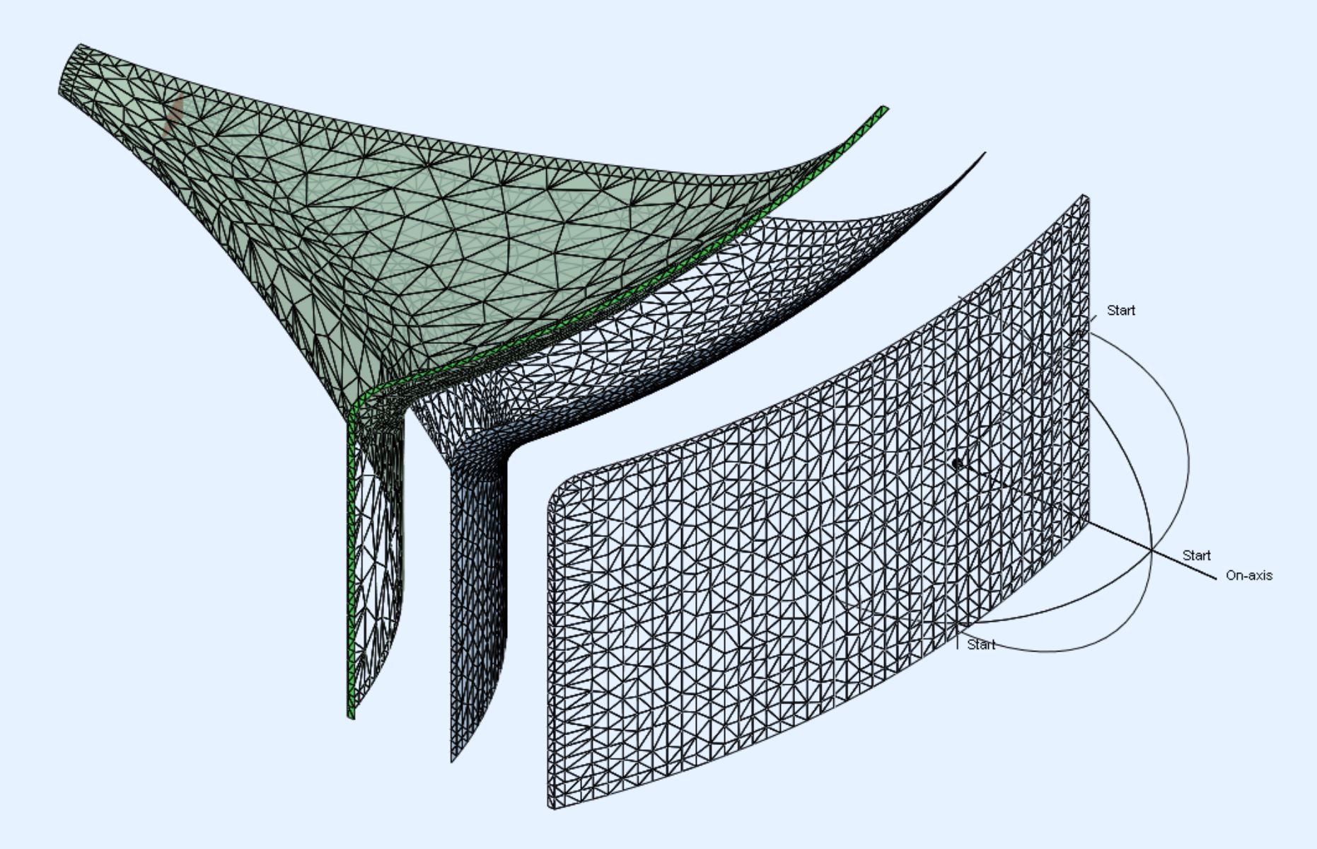
I would like to thank DonVK again for his support and discussions regarding BEM simulation. My calculators generally put out a point cloud which can be used to generate a mesh. Since I don’t use any external software to generate the point cloud, I can tell you that every single damn point is the result of a mathematical operation that of course had to be programmed. This is quite cumbersome, since threshold values ​​also have to be inserted in order to avoid points that are too close or too distant. However, the new radial like algorithm is ideally predestined for BEM simulations, because only 1/4 of the points have to be calculated and the remaining points result from symmetry operations. In a slightly modified form compared to a point cloud for a complete horn I am now able to calculate and export the corresponding point clouds in 1/4th symmetry for the individual BEM elements directly from the program code. With an appropriate AKABAK template project file only a few modifications are necessary each time to create a new project.

Simulations do not have to follow size and cost restrictions in reality. But if we can make it large to work good then we can also make it small to work good.

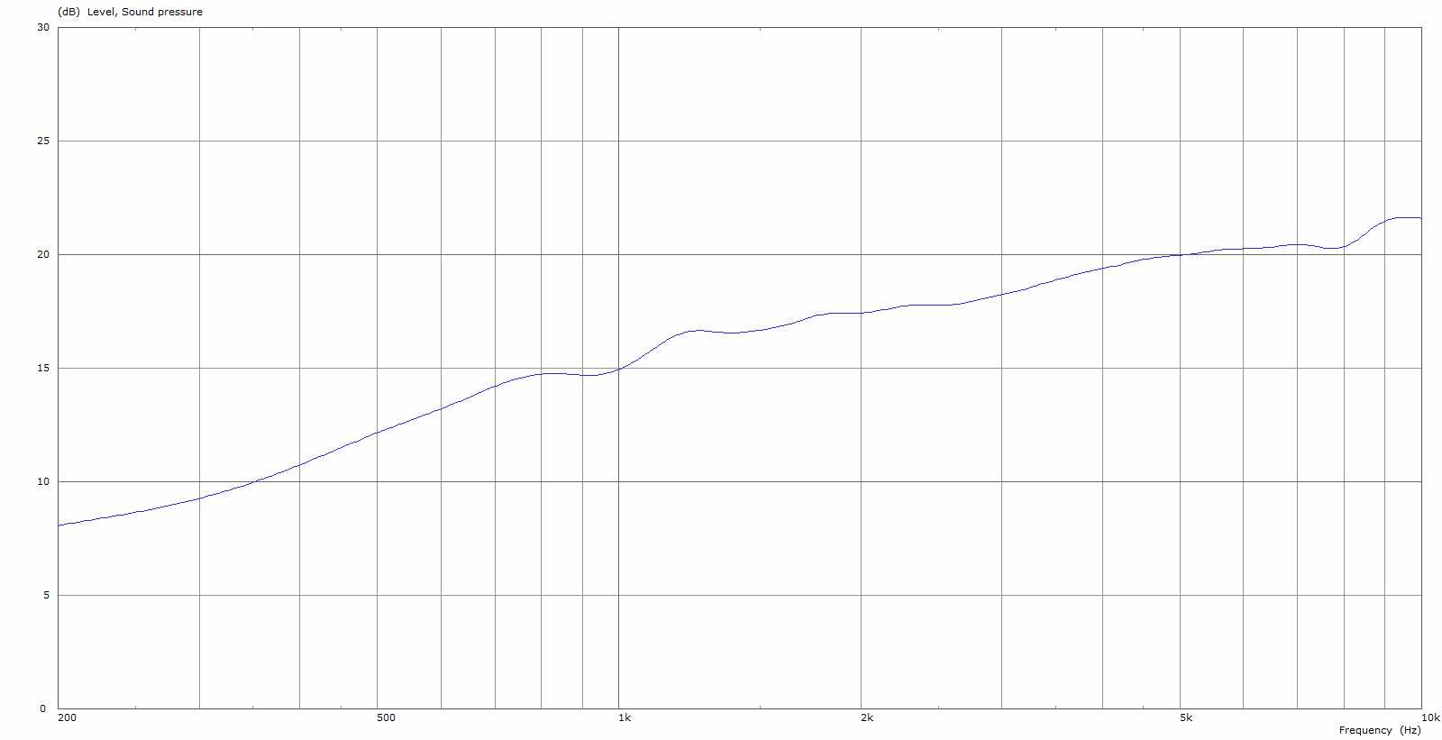
Let us begin with the results of the radiation impedance of this large waveguide:

Radiation Impedance

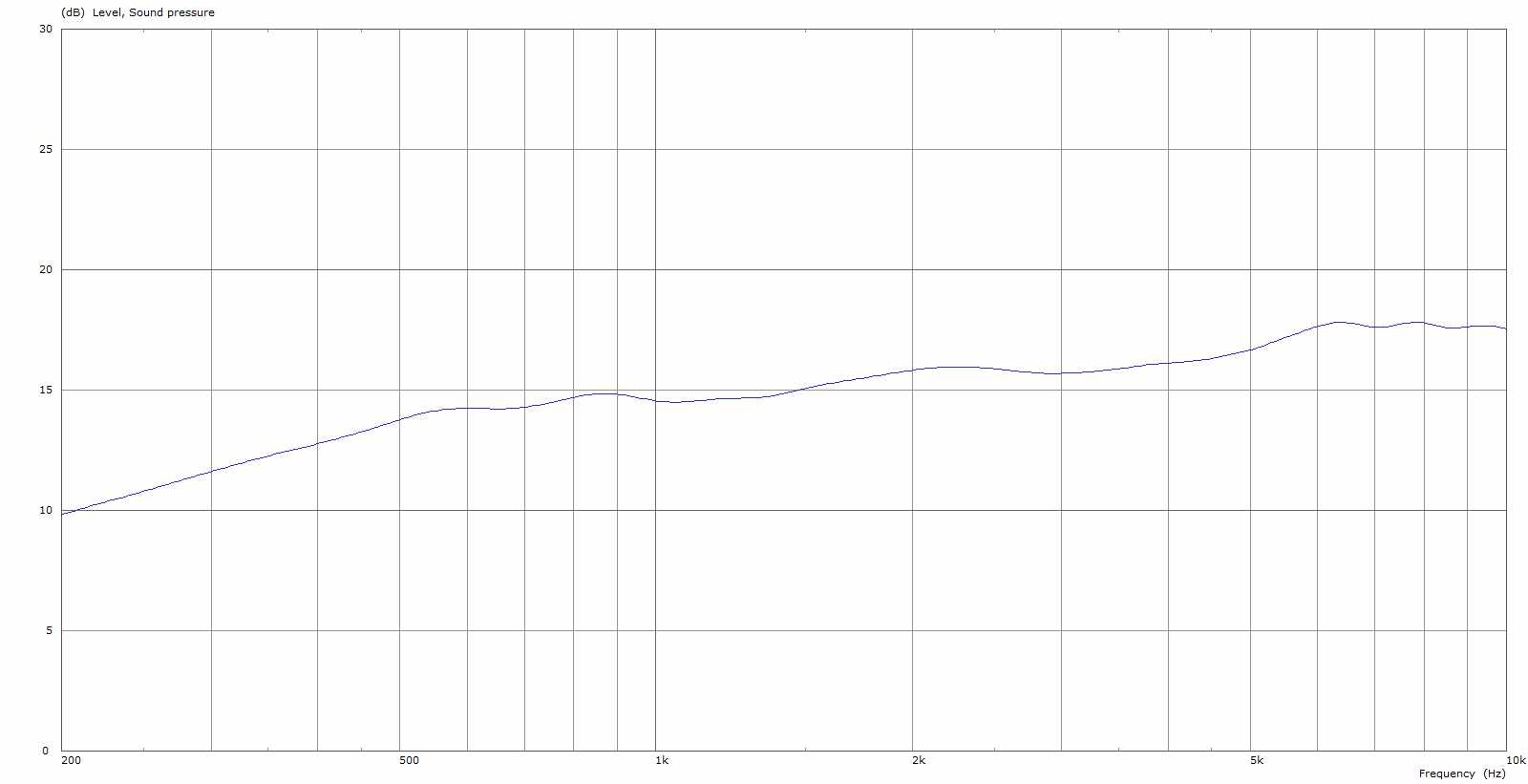
This was really surprising to me how low the loading capabilities are going and the absence of any considerable peaks and with a very smooth decay. The horizontal power response is also very smooth:

Power Response

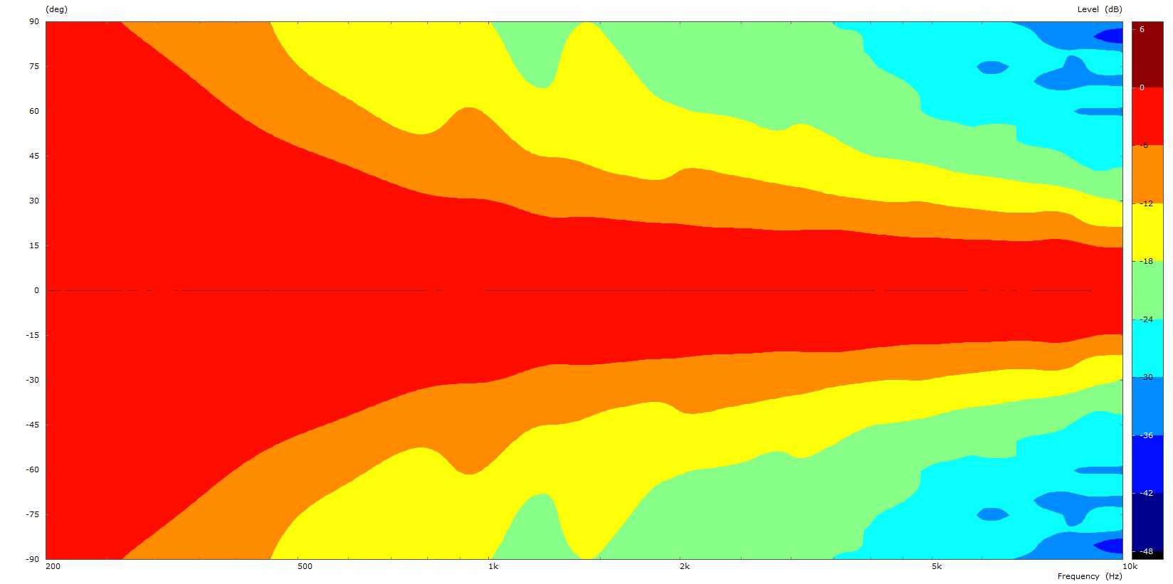
What I personally find excellent are the horizontal and vertical polar. One of the best performances I reached so far:

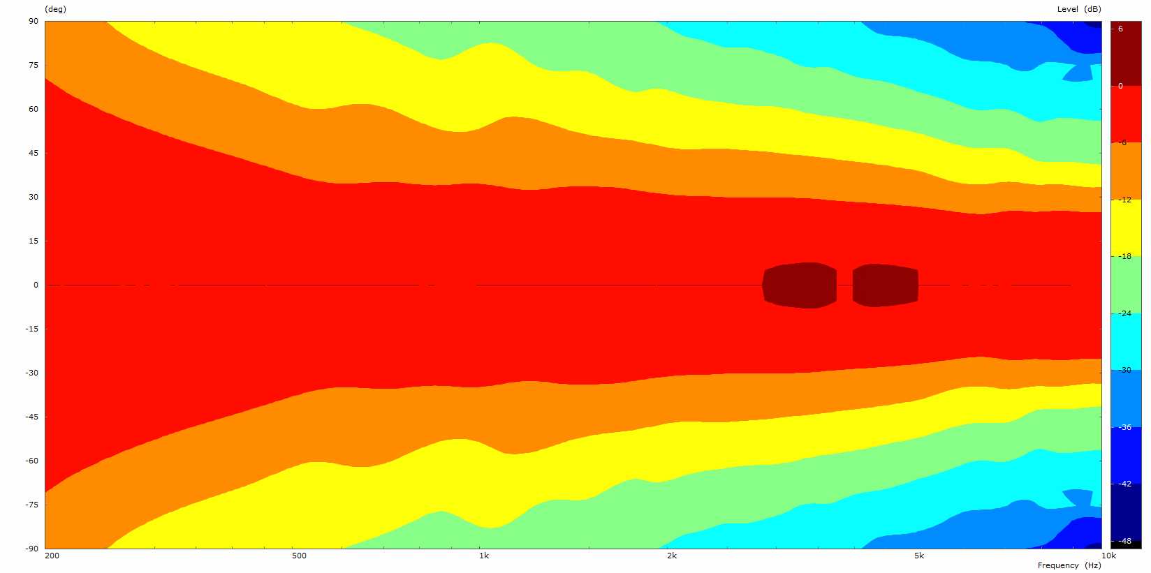
WN horizontal radiation polar (6dB step)

WN vertical radiation polar (6dB step)

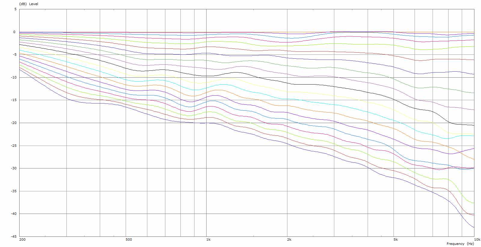
WN horizontal polar (0-90, 5 degrees step)

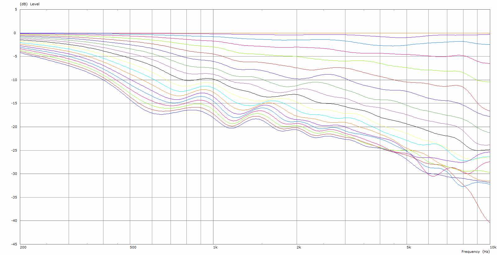
WN vertical polar (0-90, 5 degrees step)

I am very satisfied with the results. The horizontal dispersion is almost constant directivity with control down to about 500Hz. Over all a very smooth behaviour for a 2″ horn up to 10k which I had not expected at start. The performance could even be improved by adding a small round over at mouth which would normally exists for a real incarnation. Bear also in mind that the computation time took several hours on a powerful computer. The mesh resolution required for higher frequencies (>10kHz) simulation would take significantly more RAM and more CPU time to solve. For the sake of completeness here are the two directivity indexes  (DI) which have a nearly linear behaviour and slightly increase which looks like a very nice performance to me:

Horizontal DI90

Vertical DI90

I am really happy with the results especially the good directivity control surprised me a lot. The end flares are doing a good job because the normally typical midrange narrow seems to absent here. The results encouraged me to use the Neile parabola for a horn that respects exponential loading while preserving much of this directivity control. But this is another story…