++ Important Update ++
This design is obsolete and surpassed by my final generation William Neile horn series:
Final Generation William Neile Acoustic Loading Horn Series – Part I
The corresponding calculators are no more available! Any permission for the free use of my Calculators, designs and any of my IP have been revoked! Please read here:
https://sphericalhorns.net/news_announcements/
==================================================================
I find it difficult to formulate the appropriate introductory words for a person like Jean-Michel Le Cléac’h (JMLC). Unfortunately, I didn’t have the opportunity to discuss my work with him, although theoretically it would have been possible but my interest in horns arose just a few years ago. I would have been honoured to have received feedback on my work from Jean-Michel.
Recently, I realized what meaning as human being Jean-Michel Le Cléac’h must have had for other people when I recognized that Bjørn Kolbrek and Thomas Dunker dedicated their excellent book about “High-Quality Horn Loudspeakers Systems” to him.
Here are two links to diyaudio.com for those who are not so familiar with his work and his life: Link1, Link2.
Interestingly, JMLC emphasized that we should understand his work on horns more as a method to calculate horn profiles than rather a new expansion. This is exactly how I understand it and this post will describe my implementation of JMLC’s method.
I don’t want to claim that my algorithm delivers exactly the same results as the original JMLC spreadsheets, which can still partially to be found in the web, because my approach is based on the actual numerical summation of a fixed growing conical mid element with distinct opening angle and all outer growing surface area elements for the approximated curved wave fronts. The most outer element for each step is added to fulfil the given expansion law. The individual compound construction wave fronts for a given radius are numerically approximated by a spherical cap for conical the mid element similar to the spherical wave horn and the surface areas of all conical frustums (Link_Wolfram_Mathworld) for the outer growing and most outer elements. The base assumption is that each iterated element is normal to the previous element until the horn wall is reached with the newly to added most outer element which is also normal to the horn wall. This sounds complicated but some drawings might help for a better understanding:
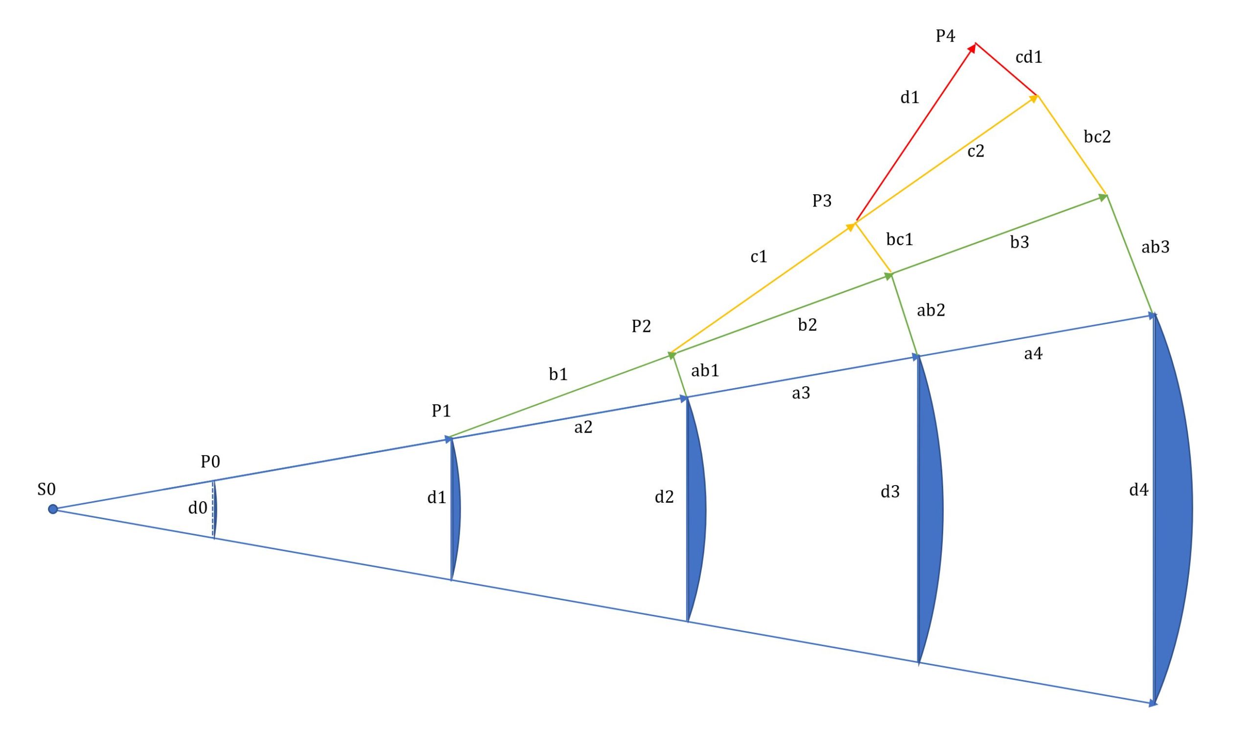
With help of this drawing as base template I programmed the algorithm in VBA. This might be different to the descriptions that can be found elsewhere. Basically everything starts with the virtual sound source at s_0. The throat or the beginning of the horn with the diameter d_0 is located at P_0. From s_0 via P_0 to P_1 the conical base element is created, which also determines the opening angle of the horn. This conical base element expands approximately linear along the horn axis. The assumed wave front is a spherical cap which is defined by the expanding wave front radius and the opening angle at each stepped point. If we assume an exponential expansion law for the wave front surface areas we need to correct the conical base element by adding an additional element from a distinct point on. In my approach the first outer element to be added arises from P_1 to P_2 and not from P_0 toP_1. Why did I do it like that? A minor reason is numerical stability. But we have a constraint here which is the given expansion law of the wave front surface area along the horn axis which can be written as:
\tag{1a}S_z = S_0\cdot \left( cosh(\frac{m}{2}\cdot z) + T \cdot sinh(\frac{m}{2}\cdot z) \right)^2
\tag{1b}m=\frac{4\pi \cdot f_c}{c_s}
The only reasonable implementation for the first conical element is that it exactly fulfils the pre-defined expansion law for the selected step size – to whatever this expansion law was defined to. This also means that the expansion law defines the opening angle of the horn, s_0 and r_0 (the initial virtual wave front radius). The only way to get another opening angle is therefore to change the T-factor or use the PETF method described in a recent post. Otherwise, if the opening was set too large the next outer element must be negative or if set to small the next outer element would correct the missing surface area which makes no sense.
Another different approach to implement JMLC’s method which is shown in the next picture and for some readers it might look more familiar:
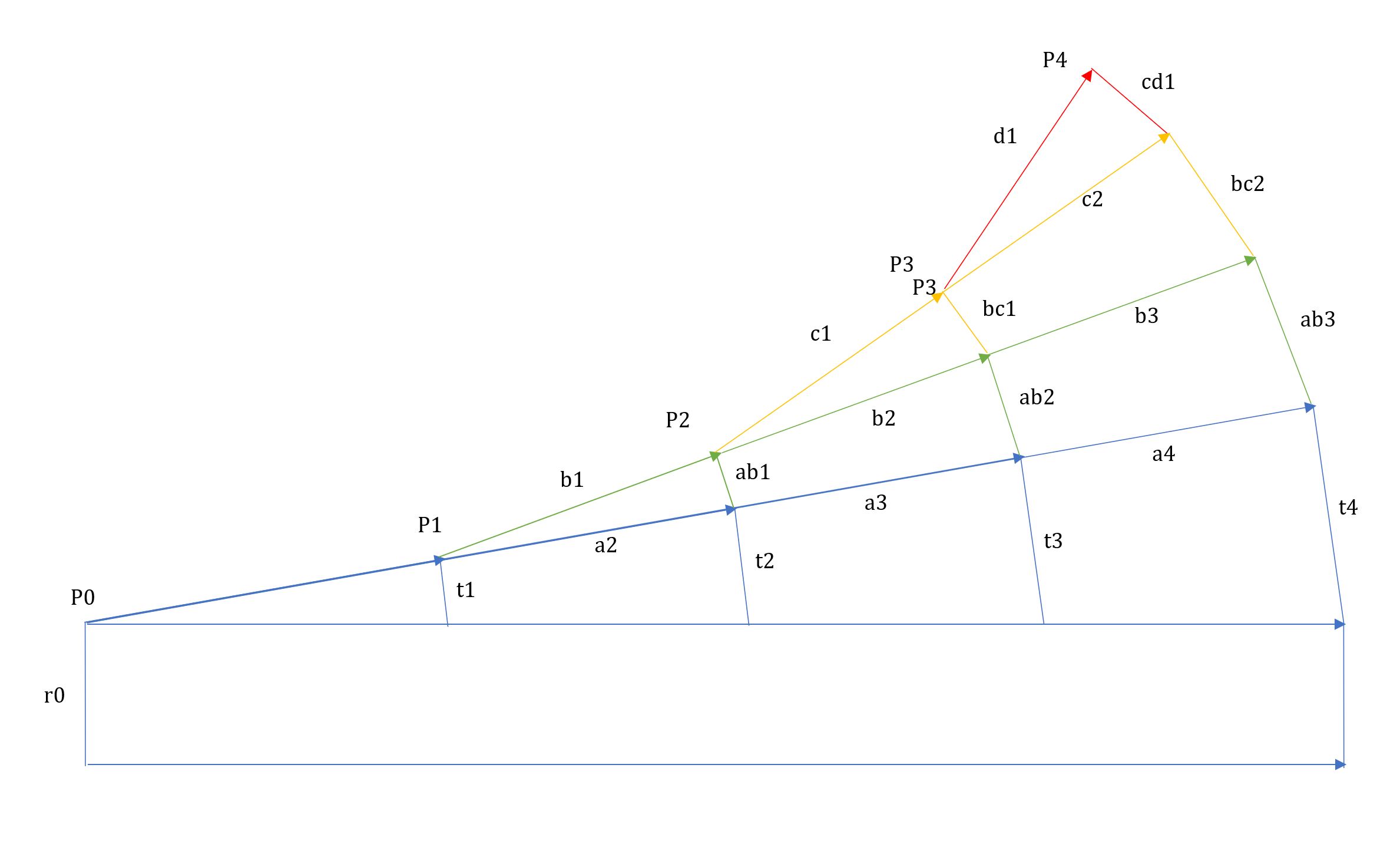
Here, the inner element remains flat which is the best solution in contrary to make is a spherical cap. In this way it will define the top of the wave front which is flat for diameter d_0 and it’s surface area is simply defined by the throat radius. The first added element defines the opening angle of the horn but still as constraint of the underlying expansion law. I have implemented both versions but decided to use the first. The corresponding start values can be calculated by a Newton optimization with reasonable start parameters the algorithm converges quite well. Although, my calculator is not fool-proof, so bad parameters could prevent a successful run.
The base for any later modifications within my calculator is always the round horn to determine the construction wave front surface areas and the resulting horn profile. With the vectors and angles shown in the next picture it is possible to calculate the first conical frustum at lcm1 as rotation around the horn axis which is at the same time the first outer element to be added for this initial step. For the next step we know the angle \alpha under which this element expands and therefore we know lcm2. Summing up the surface areas of the inner element and lcm2 will be smaller than S_z. An outer outer element need to be added to compensate the difference which defines bc1. The next steps continue this procedure each with one more known expanding element and one missing outer element to account for S_z:
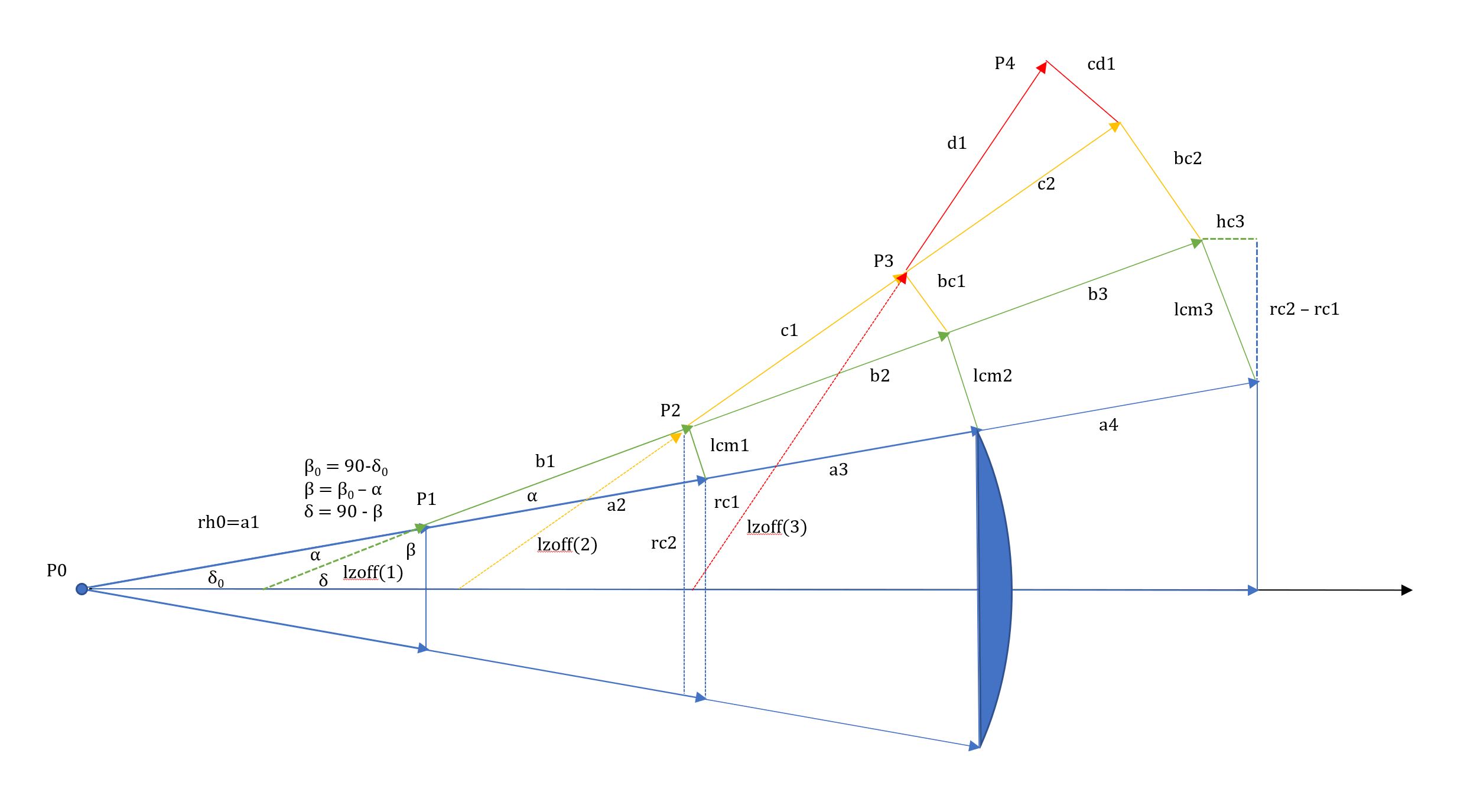
In order to keep the algorithm numerically robust there is a maximum angular step size defined in the code to calculate each conical frustum more precisely as sum of several smaller conical frustums. This becomes more and more important for the expanding elements as from the drawing they look like a straight line but in fact they need to be curved. The straight arc length would under-estimate the surface area. I am quite confident to having found a numerically robust and precise algorithm to calculate each element with sufficient precision independent of the angle of an element. What might become a problem if the T-factor is changing very fast within a few steps.
With T=1 we get very similar looking horn profiles than the original JMLC profiles:
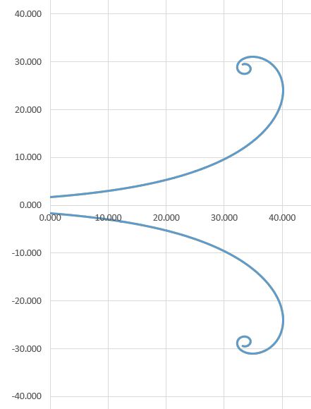
JMLC inspired with cut-off 300Hz
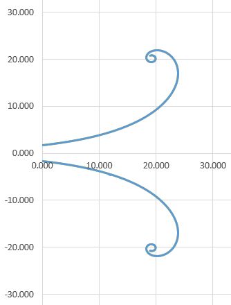
JMLC inspired with cut-off 425Hz
In order to emphasize this point again, the opening angle for each horn profile with my JMLC inspired calculator is an intrinsic property of the chosen cut-off value or T_0-factor. To increase the opening angle either use an higher cut-off value or a larger T-factor.
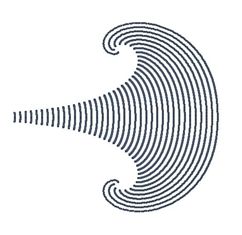
At least for me it is always very interesting to see the underlying construction wave fronts for a horn profile. It should be noted that the following construction wave fronts are normal to the horn walls:
My calculators are intended to export a point cloud for each calculated horn profile. If we go for a round JMLC horn there is nothing really new. Anyway, I will show such a round horn with 300Hz cut-off as result of my calculator as mesh file with a roll-back terminated at 180 degrees:
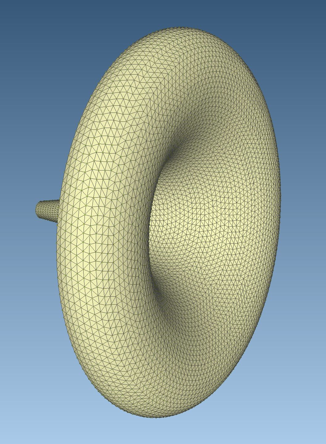
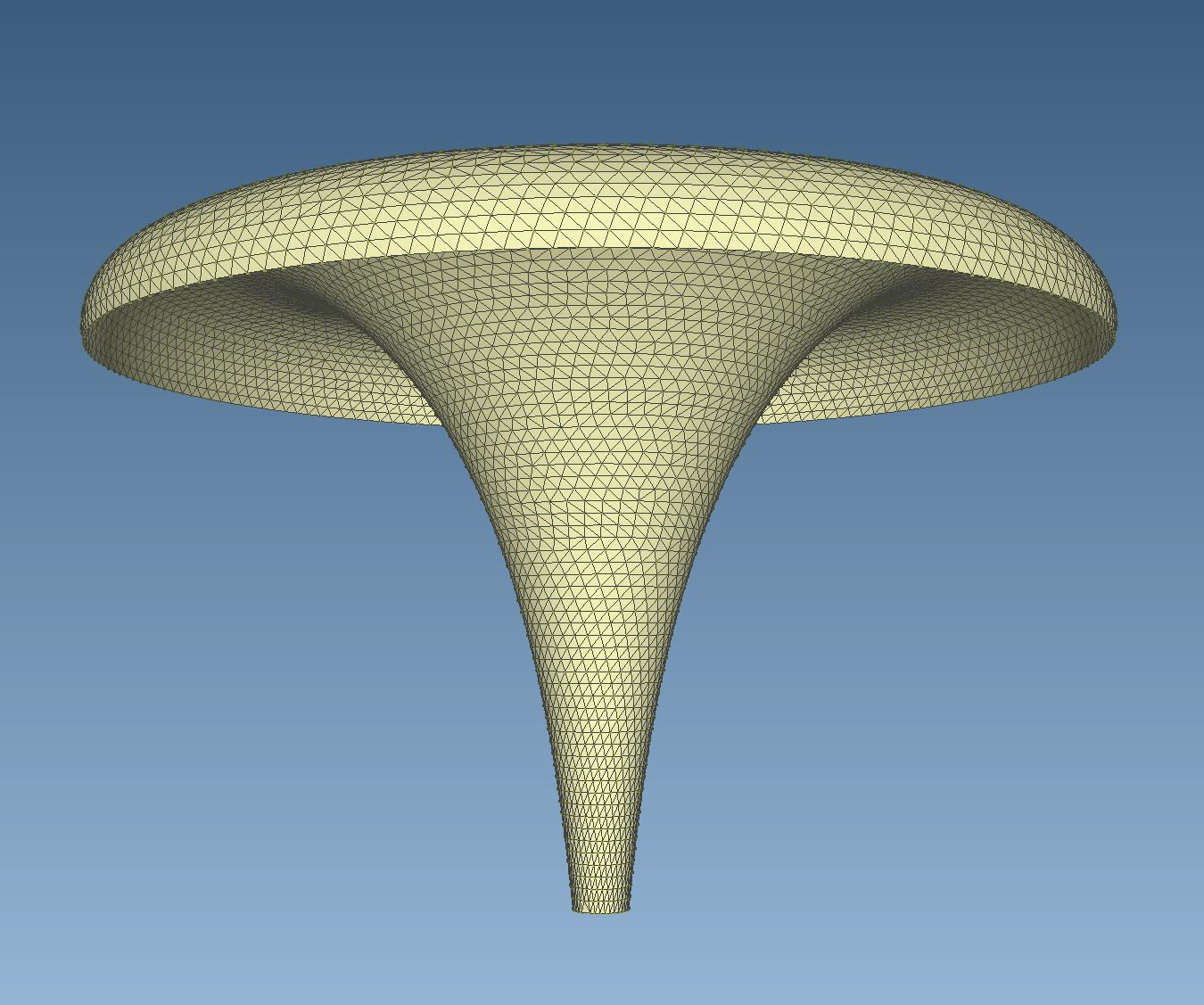
For a 425Hz/1.4″ round horn an STL file is additionally attached to this post jmlc_425_14i_rnd which can be opened with an appropriate 3D viewer like MeshLab.
I have decided to publish this JMLC inspired calculator and also provide some of my extensions like PETF. If horizontal and vertical expansion PETF parameters are set to the same values a round horn will result as just shown. If set differently many other nicely looking horn shapes shapes are possible. Especially this profiles look very appealing to me:
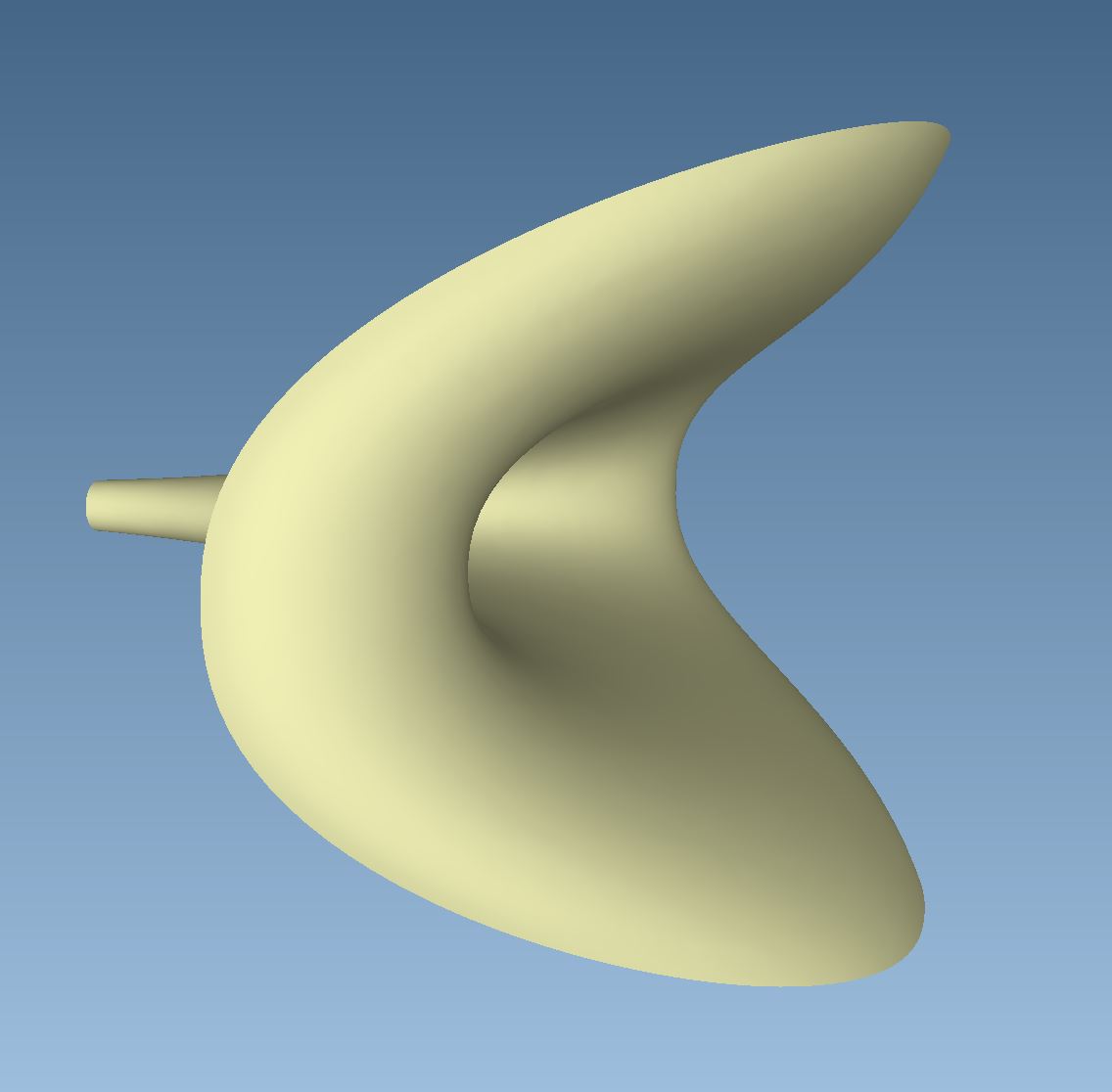
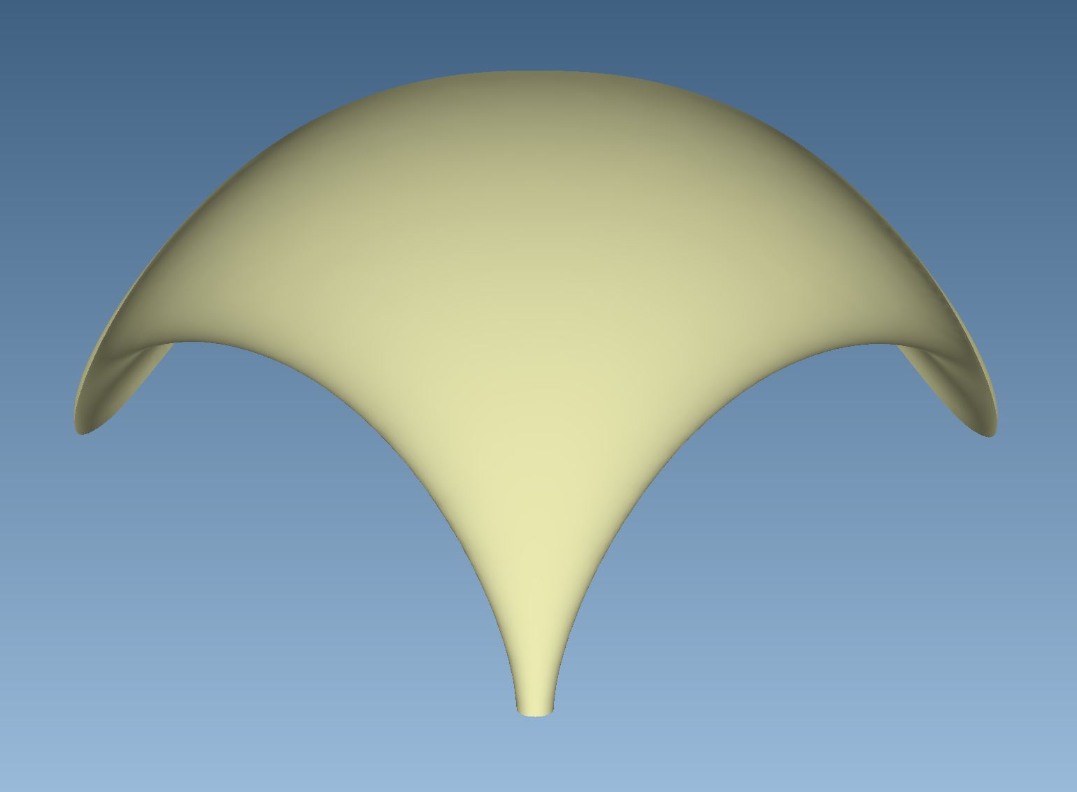
This sort of horn shape using different hrz/vrt expansion was already presented at diyaudio.com forum some time ago and denoted as hvdiff at that time: Link_diyaudio_com_hvdiff.
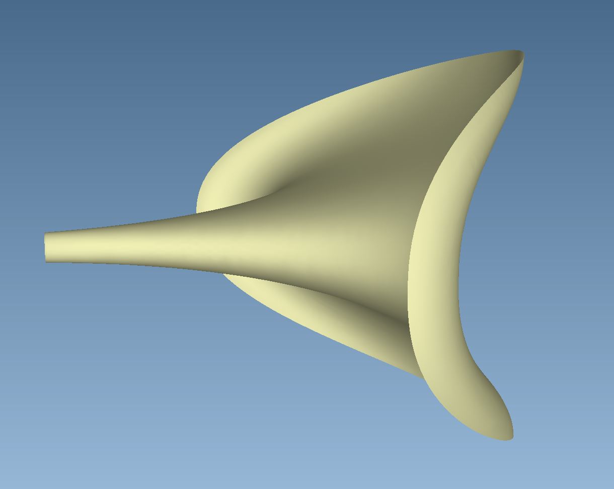
By varying the Lamé exponent a transition from round to square is possible. Here is an example of Lamé exponent of 4.0 for a 425Hz horn with equal PETF settings:
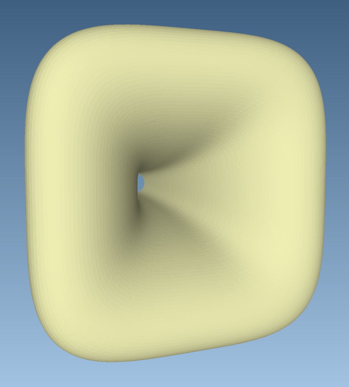

The actual JMLC inspired horn calculator spreadsheet is located in the Download section of my page. Have fun with it and maybe some day we see a real printed horn as result of my work.